Numerical Experiments and Analysis of Shock Wave Diffraction around Structures

1. INTRODUCTION

The interest of studying transient shock wave flows around solid bodies is motivated by the need to understand the physics of gas-dynamic phenomena. The present study helps engineers to improve the design performance of structure exposed to blast waves or high-speed supersonic vehicles. Shock wave diffractions over solid structures have been comprehensively investigated, but the mechanism of such complex shock dynamics is still a challenge and still not fully understood (i.e. the onset of Kelvin–Helmholtz shear layer instability). The diffractions reveal complex unsteady flow associated with flow separation and complex interaction systems. The flow separation is defined as the detachment of fluid flow from the solid structure due to a sharp edge (i.e. backward-facing step) or to the formation of an adverse pressure gradient (i.e. curved structure).

It has been found that the numerical solutions of the inviscid solver reproduce accurately shock propagations, reflections, and interactions.^1–6 This is because the compressible flows have inviscid characteristics. It was also shown that there is no difference between the flow features based on the inviscid and laminar solvers applied to shock wave diffraction over the backward-facing step.^7–9 The justification for using a laminar solver for compressible flows is that the Reynolds number effect is trivial or is not entirely appropriate as the flow has inviscid characteristics. Moreover, it has sufficient numerical (artificial) viscosity which reduces as the mesh resolution is increased.¹⁰ Inviscid and viscous simulations are effective in capturing most of the large-scale features. However, they fail to reproduce the fine-scale features and boundary layer separation under increasingly adverse pressure gradient due to insufficient numerical viscosity.^10–12 Recently, Chaudhuri and Jacobs⁵ have developed an artificial viscosity Galerkin method based on Euler equations which resolved even the fine-scale details of shock wave dynamics. Unfortunately, they have not examined the method for boundary layer separation. The turbulent solver has proven to be highly successful for the adverse pressure gradient flows.^10,13

On the other hand, unlike sharp corners, there have been relatively little experimental investigations on the diffraction of shock waves over curved structures.^{e.g. 13–15} The experimental shadowgraph and schlieren images have not resolved fine-scale features due to the limitations of the flow imaging system.¹⁵ The curved surface enhances the adverse pressure gradient by the continuous variation of the surface boundary condition,¹³ consequently, it is more challenging to simulate numerically. This could be due to the difficulty in predicting the location of the separation point, which has a dominant effect on the flow development. Moreover, the curved splitter flow is not self-similar in time because it contains a length scale (curve radius). However, some numerical investigations also have been performed using a laminar solver¹⁵ and turbulent solver.¹³

The objectives of the research are twofold. One is to verify whether the inviscid solver can simulate the shock wave diffraction in the presence of the adverse pressure gradient and flow separation. The second objective is to evaluate the addition of viscosity (laminar solver) and turbulence (turbulent solver) under more demanding conditions such as compressible flow separation, especially in the presence of adverse pressure gradient. The manuscript is organized as follows. In section two, the problem setup for the present study is illustrated. A brief description of the governing equations, the turbulent model, and the numerical method is described in the third section. The qualitative and quantitative results of the three cases are discussed in section four. Finally, the conclusions are drawn in section five.

2. Problem Definition

Extensive numerical experiments have been performed and assessed for complex compressible flows associated with separation and shear layer generation. The investigation has been conducted using:

1. The Euler equations (inviscid solver).

2. The Navier-Stokes equations (laminar solver), and

3. The Reynolds averaged Navier-Stokes equations coupled with the shear-stress transport, SST, turbulence model (turbulent solver).

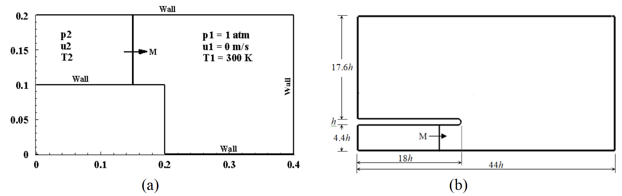
The three solvers have been validated against three test cases of shock wave diffraction over backward-facing step, sharp and curved splitters. The study cases are selected because their evolving flows reveal discernible distinct behavior. The geometry and flow condition of the three cases under investigation are shown in Fig. 1. For all cases, an incident planar shock wave of Mach number, M, moves from left to right into an ambient air at rest, Fig. 1. Supersonic flow and non-reflecting boundary conditions are specified at the inlet and outlet sections, respectively.

The supersonic speeds of an incident Mach numbers (M= 1.31 and 2.4) around solid bodies are simulated. The two speeds produce subsonic and supersonic regions behind the incident shock wave, respectively.⁹ The post-shock flow remains subsonic for an incident Mach number less than 2.07.^10,16 As the shock intensity increases, the developing flow grows into a more complex system and produces additional features. Supersonic post-shock flow (M > 2.07) produces distinguished evolving flows.^3,16 It is worth mentioning that there are no additional flow features appear for Mach numbers greater than 3.0.¹⁷ Moreover, the two Mach numbers (M = 1.31 and 2.4) are selected due to the availability of experimental results^15,18 which can be used to validate the present numerical models.

For the first test case, Fig. 1a, the shock wave of Mach number, M=2.4, moves over the backward-facing step (90^o sharp corner) according to the experimental setup of Van Dyke.¹⁸ The upper and lower boundaries are rigid non-penetrable walls. The initial conditions behind the shock front are specified in the region between x = 0 and x = 0.15, as shown in Fig. 1. The second and the third test cases are shock wave with Mach number, M=1.31, diffracts around convex 8o sharp and curved splitters, respectively, Fig. 1. The splitters have height, h, of 5.63mm similar to the experimental setup of Gnani et al.,¹⁴ Fig. 1. The splitters have a length of 18h. The sharp splitter has a wedge angle of 8^o. As shown in Fig. 1, the computational domain covers the area 44h long and 23h high. The side, upper and lower boundaries are non-reflecting boundary conditions to reduce waves reflected.

Fig. 1.Geometry and flow conditions

(a) Backward-facing step; (b) Splitter

3. Computational Fluid Dynamics

3.1. Governing Equations

The two-dimensional Navier–Stokes continuity, x-momentum, y-momentum, and energy equations can be written as:

\[\frac{\partial\rho}{\partial t} + \frac{\partial}{\partial t}\left( ρu \right) + \frac{\partial}{\partial t}\left( ρv \right) = 0 \tag{1}\]

\[\begin{align} &\frac{\partial}{\partial t}\left( ρu \right) + \frac{\partial}{\partial x}\left( \rho u^{2} + p \right) + \frac{\partial}{\partial y}\left( ρuv \right) \\ &= \frac{\partial\tau_{xx}}{\partial x} + \frac{\partial\tau_{xy}}{\partial y} \end{align} \tag{2}\]

\[\begin{align} &\frac{\partial}{\partial t}\left( ρv \right) + \frac{\partial}{\partial x}\left( ρuv \right) + \frac{\partial}{\partial y}\left( \rho v^{2} + p \right) \\ &= \frac{\partial\tau_{xy}}{\partial x} + \frac{\partial\tau_{yy}}{\partial y} \end{align} \tag{3}\]

\[\begin{align} &\frac{\partial}{\partial t}\left( ρe \right) + \frac{\partial}{\partial x}(\rho e + p)u + \frac{\partial}{\partial y}(\rho e + p)v \\ &= \frac{\partial}{\partial x}\left( u\tau_{xx} + v\tau_{xy} \right) + \frac{\partial}{\partial y}\left( u\tau_{xy} + v\tau_{yy} \right) \\ &\quad - \frac{\partial q_{x}}{\partial x} - \frac{\partial q_{y}}{\partial y} \end{align} \tag{4}\]

Where ρ is the density, u and v are the velocity components, and e is the total energy. The stress terms can be expanding by using laminar fluid viscosity, µ:

\[\begin{align} \tau_{xx} &= \frac{2\mu}{3}\left( 2\frac{\partial u}{\partial x} - \frac{\partial v}{\partial y} \right), \\ \tau_{yy} &= \frac{2\mu}{3}\left( 2\frac{\partial v}{\partial y} - \frac{\partial u}{\partial x} \right), \\ \tau_{xy} &= \mu\left( \frac{\partial u}{\partial y} - \frac{\partial v}{\partial x} \right) \end{align} \tag{5}\]

The heat conduction can be expressed in terms of the temperature, T, and thermal conductivity, k, by:

\[q_{x} = - k \times \frac{\partial T}{\partial x},\ q_{y} = - k \times \frac{\partial T}{\partial y} \tag{6}\]

The energy, e, is given in term of internal energy, i, by:

\[e = \rho i + \frac{u^{2} + v^{2}}{2} \tag{7}\]

The pressure, p, is defined by the ideal gas equation of state since T< 2000K (weak shock wave):

\[p = \rho RT \tag{8}\]

For a constant ratio of specific heats (γ=1.4) and the assumption of a perfect gas, the internal energy, i, can be calculated from:

\[\rho i = \frac{p}{\gamma - 1} \tag{9}\]

3.2. Turbulence Model

The SST turbulence model is selected because it combines near-wall accuracy and the free stream robustness.¹⁹ For the SST turbulence model, the equations for the turbulence kinetic energy, k, and dissipation rate,ω, are solved¹⁹:

\[\begin{align} &\frac{\partial}{\partial t} \left( \rho k \right) + \frac{\partial}{\partial x} \left( \rho u k \right) + \frac{\partial}{\partial y} \left( \rho v k \right) \\ &= \frac{\partial}{\partial x_j} \left( \Gamma_k \frac{\partial k}{\partial x_j} \right) + G_k - Y_k \end{align} \tag{10}\]

\[\begin{align} &\frac{\partial}{\partial t} \left( \rho \omega \right) + \frac{\partial}{\partial x} \left( \rho u \omega \right) + \frac{\partial}{\partial y} \left( \rho v \omega \right) \\ &= \frac{\partial}{\partial x_j} \left( \Gamma_{\omega} \frac{\partial \omega}{\partial x_j} \right) + G_{\omega} - Y_{\omega} + D_{\omega} \end{align} \tag{11}\]

The terms Γ, G, Υ, D, represents the effective diffusivity, generation, dissipation, cross-diffusion, respectively, of the turbulence kinetic energy, k, and the dissipation rate,ω.

3.3. Numerical Methods

The computational fluid dynamics reveals the precise prediction of transient shock wave around structures. A variety of numerical solvers with high-order accuracy have been proposed which provide good results on complicated physical systems.^9,20 However, the selection of the appropriate numerical solver is a challenging process. One of the challenges in the numerical simulation of compressible flows is to eliminate the numerical uncertainties due to cell size and solver resolution. A low-order solver can give a severely over-damped solution, resulting in sharp gradients being spread out which is not suitable for the computation of moving discontinuities. However, if a higher-order solver is used, sharp gradients can be over-predicted and underdamped leading to non-physical oscillations.²¹

The above governing equations are numerically solved by a finite volume method. The flow is modeled using a second-order ASUM+ upwind scheme.²² The AUSM+ requires the initial values of flow variables at the faces of cells. A second-order least-squares cell-based scheme has been selected for the flow spatial discretization where the gradients are estimated within each cell, and then the face values are obtained. The non-differentiable limiter, which maintains stability in the upwind discretization schemes, is used.²³ The density-based solver in conjunction with Gauss-Seidel linear equation solver is employed. The transient terms are discretized by first-order explicit time which shows poor convergence and large nonphysical oscillations at discontinuities. The CFL is set to a low number of 0.5 to reduce non-physical oscillations.

Fig. 2.Schlieren and corresponding mesh

(a) Pressure-gradient adaptation (3 levels); (b) Density-gradient adaptation (3 levels); and (c) Density-gradient adaptation (5 levels).

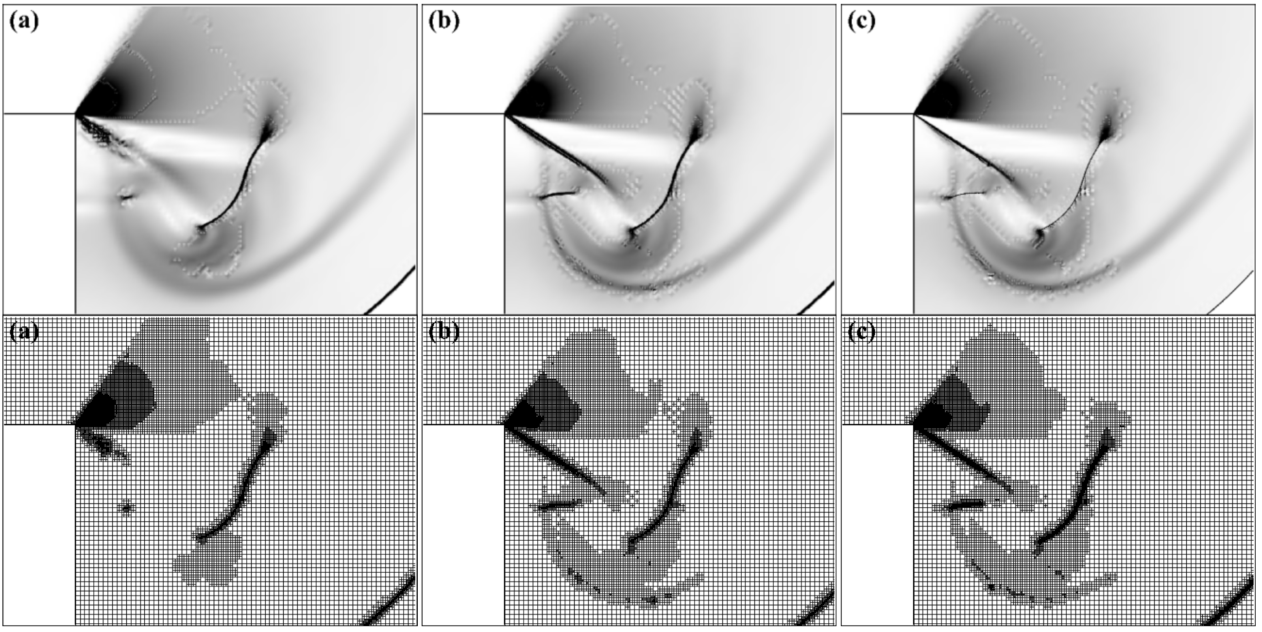
The flow domains are discretized using quadrilateral mesh. An initial cell size of 1mm² is utilized in the whole computational domains. It is revealing mesh size of 60,000 and 32,345 cells for the backward-facing step and sharp splitter, respectively. However, for curved splitter, initial cells of the size 1×10^-2mm² are clustered to the curved surface in the region of the vortical structure to predict the boundary layer in the viscous computations, it yields an initial mesh size of 36,457 cells. It is found that the employed initial cell size proves adequate for capture shock wave, vortex, and shear layer development when coupled with dynamic mesh adaption. The mesh is adaptively refined to five times in zones where gradients exceed 5%. Refining one cell involves halving both the horizontal and vertical mesh size, leading to the creation of four new cells. In the contrast, the mesh is coarsened where the gradient is below the lower threshold of 2% which means that the important flow features have passed away. The mesh adaption based on the density gradients proves to be better than the pressure gradients adaption, Fig. 2. The preliminary numerical experiments shown in Fig. 2 confirm a strong mesh independency.

4. Results and Discussion

4.1. Backward-facing Step

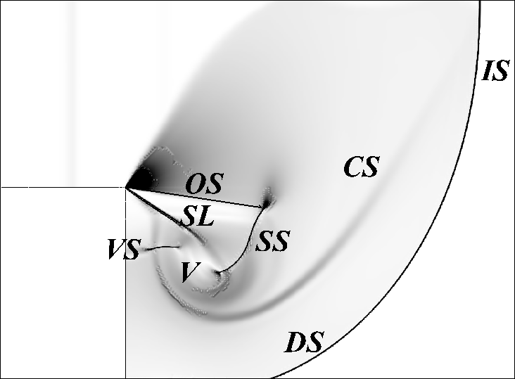
As a planar shock wave moves over a backward-facing step, a complex flow structure develops over time. The small-scale shock tube experiments showed that the developed flow field was self-similar.¹⁷ Recently it was demonstrated, by using large-scale experimental facilities, that the flow was temporally not self-similar.¹⁶ The resulting flow depends on the strength of the incident shock wave. However, the general flow features of incident shock, IS, of Mach number, M =2.4, diffraction over backward-facing step, are shown in Fig. 3 as reported by the experimental results of Dyke.¹⁸ The curved diffracted shock, DS, is separated due to the presence of the sharp corner and propagates downwards normally to the wall. A reflected expansion wave, EW, travels upstream into the post-shock region. The separated shear layer, SL, rolls up into a spiral vortex, V, downstream of the sharp corner per Fig. 3. The contact surface, CS, moves forward behind the incident shock. Its lower end is dragged around the vortex structure. The shock-shock and shock-vortex interactions generate vortex embedded shocks, VS, and horizontal oblique shock, OS, above the shear layer, starting from the separation point as shown in Fig. 3.³ It is connected to a vertical second shock, SS, that ending at the vortex core.

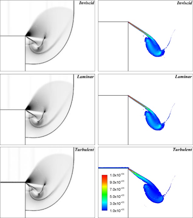
The numerical schlieren and vorticity magnitude of different solvers, at the time 125μs after the incident shock arriving at the sharp corner, are shown in Figs. 3 and 4. It is found that all solvers reveal excellent qualitative agreement with the corresponding experimental shadowgraph.¹⁸ The trivial flow details of the resulting complexity flow in terms of shape, size, and position are well captured, Figs. 3 and 4. Figure 5 shows the pressure area-weighted average at backward-facing step surfaces. The average pressure is normalized by the shock pressure which is 6.55 at Mach number M=2.4. The quantitative analysis shows that the turbulent solver produces a slightly 0.2% higher pressure load than the inviscid and laminar solvers.

Fig. 3.Schlieren showing flow features of shock wave diffraction over a backward-facing step.

IS: incident shock, DS: diffracted shock, CS: contact surface, SL: shear layer, V: vortex, OS: oblique shock, SS: second shock, and VS: vortex shock.

4.2. Sharp Splitter

Flow separation is the general flow feature of weak shock wave of M=1.31 diffraction around 172^o sharp splitter. The generated shear layer rolls up into a vortical structure downstream of the splitter as shown in Fig. 6. With the flow evolution, an interesting feature that the Kelvin–Helmholtz, KH, instability is developed on the shear layer surrounding the vortex, see Fig. 6. It is associated with the roll-up of small vortices along the shear layer, SL. This can be attributed to the perturbation of the shear layer by the contact surface, CS, interaction which makes the shear layer unstable forming a series of small vortices rolling-up with the main vortex.⁴ Similar instability was previously observed experimentally.^14–16 and numerically.^5,9 Numerical schlieren and vorticity magnitude maps at 140μs after the incident shock arriving at the sharp corner for different solvers are presented in Fig. 6. The inviscid and laminar solvers reveal the KH instability which is more pronounced at the laminar solver which produces more small vortices with higher vorticity magnitude, consequently, more spinning motion, Fig. 6. The additional dissipation of the turbulent solver stabilizes the shear layer. Moreover, the turbulent solver produces less vorticity in the core of the main vorticity structure, Fig. 6.

4.3. Curved Splitter

Shock wave diffraction around curved splitter poses a sufficiently strong challenge to be simulated due to the boundary layer separation of strong adverse pressure gradient. As shown in Fig. 7, in addition to the flow feature of the previous case, the shock wave of M = 1.31 diffraction around curved splitter exhibits lambda shocks, TL. The lambda shocks, TL, comprise a series of triangle-shaped shocks around the downstream edge of the shear layer, SL, starting from the separation point. The present numerical schlieren shown in Fig. 7 agrees well with the experimental shadowgraph of Quinn.¹⁵

Fig. 4.Schlieren (left) and vorticity (right) of shock wave diffraction over the backward-facing step for different solvers.

Fig. 5.Time evolution of the normalized average pressure at the backward-facing step surface for different solvers.

The results of the shock wave of M = 1.31 diffraction around curved splitter for different solvers are presented in Figs. 8 and 9. It is obvious that, as demonstrated by the frames at time 60μs after the arrival of shock at the apex curve, the laminar and turbulent solvers reproduce the boundary-layer separation, which is not resolved by the inviscid solver. This can be attributed to the lack of sensitivity of the inviscid solver to the adverse pressure gradients developed on the curved wall, Figs. 8 and 9. However, similar to the experiment, the laminar solver exhibits a small secondary vortex above the splitter end of the curvature, see Fig. 9. Moreover, the flow exhibits the creation of lambda shocks, TL, early. Later on, at time 80μs, the results of the laminar and turbulent solvers show development of the vortex structure which is created by the rolling-up of the shear layer, as shown in Fig. 8.

Fig. 6.Schlieren (left) and vorticity (right) of shock wave diffraction around sharp splitter for different solvers

On the other hand, the flow structure reproduced by the inviscid solver interferes with the main flow features. However, at this point, the laminar simulation begins to depart from the experiments by creating a perturbed shear layer with a much greater level of instability in the flow. It seems that the turbulence model smoothies out the shear layer and stabilize the flow as the shear layer appears to be smooth and continuous. It is the emphasis on the importance of the turbulent dissipation on the successful longtime numerical simulation. The vortex structure is very close to the splitter which leads the vortex to entrain fluid towards its core. This leads to the creation of jet moving downward along the radius of splitter towards the beginning of curvature. The induced jet experiences an adverse pressure gradient and separates from the solid surface leading to the creation of the internal structure of the shear layer, iSL, vortex, iV , and lambda shocks, iTL.

Fig. 7.Schlieren showing flow features of shock wave diffraction around curved splitter.

SL: shear layer, V: vortex, LS: lambda shock, iSL: internal shear layer, iV: internal vortex, and iLS: internal lambda shock.

The turbulent solver predicts flow field features. The formation of all shock features is well captured numerically by the turbulent solver in terms of shape, size, and position with the shock-tube time scale. The internal shear layer, iSL, generated by the entrained fluid, agrees well with the experimental results. The flow evolution processes in the laminar solver is very similar to those in the turbulent solver, except that the vortex spiral and the internal vortex, iV, are unstable in the laminar solutions. It demonstrates that viscous dissipation in the laminar Navier-Stokes equations is underestimating the real physical dissipation which is not sufficient to damp the flow instabilities. The convection terms in the Navier-Stokes equations are discretized by the same scheme for both laminar and turbulent solvers. Therefore, the turbulent solver stabilizes the flow because of the additional turbulence dissipation in the SST turbulent model. It substitutes the low numerical dissipation of the AUSM+ which causes oscillations in the perturbed vorticity field.

Fig. 8.Schlieren sequences of shock wave diffraction around curved splitter for different solvers.

Fig. 9.Streamline (top) and vorticity (bottom) of shock wave diffraction around curved splitter corresponding to the first-raw frames of Fig. 8.

Figure 10 illustrates the angular speed of the detachment point of the boundary layer from the solid structure. Both laminar and turbulent solvers demonstrate a similar curve trend. However, the initial turbulent separation is at an angle, θ, of about 34^o, which is two degrees lower than the laminar separation angle. Moreover, the turbulent separation point travels slowly to the peak angle of 56^o, which is two degrees higher than the laminar separation point, as shown in Fig. 10. Both solvers simulate the returning of the separation point after traveling forwards to the peak angle. This can be attributed to the induced fluid moving towards the beginning of curvature, shown in Fig. 7. The induced jet enforces the separation point to return to a location earlier than the initial position, Fig. 10.

Fig. 10.Separation point location of shock wave diffraction around curved splitter for laminar and turbulent solvers.

5. Conclusions

The inviscid, laminar, and turbulent mesh-adaptive high-order numerical solvers have been implemented to investigate the unsteady flow separation process behind a diffracting shock wave over backward-facing step, sharp and curved splitters. Such flows have a wide range of engineering applications. For the two cases of the backward-facing step and sharp splitter, it is found that the addition of the viscosity and turbulence do not affect the shock wave pattern in terms of time and growing primary vortex structure. Nevertheless, it is shown that adding viscosity stimulates the Kelvin–Helmholtz instability revealed by the inviscid solver, while adding turbulence dissipation suppresses the instability without degrading the accuracy of the numerical solution.

For shock wave flows of adverse pressure gradients separation, it is found that the turbulent solver successfully reproduces the diffraction wave patterns and even the fine-scale features. Its results are in excellent agreement with the experimental shadowgraph. On the contrary, the lack of viscosity is responsible for the deviation of the inviscid and laminar solutions from the physical pattern shown by experiments. This indicates the importance of the turbulence to the flows subjected to the occurrence of a strong adverse pressure gradient to understand the shock diffraction dynamics and the associated complex boundary layer interaction physics.