1. Introduction

Wireless sensor networks (WSN) are widely used and explored in computer environments everywhere. Advances in electronics and wireless technology have led to the development of low-cost miniature sensors.¹ The smaller sensors control the integrated power because they are powered by unique batteries that are easy to replace. As a result of these restrictions, much has been done to control the sensors’ power consumption, increase their service life, and extend network life.² WSN aims to manage the environment, health services and military care. WSNs have multiple detection locations with CPU memory, but are only a short distance away. In native applications, sensors send important information to general and focal weather areas. Take each other on an Emerging Community Tour and submit verified information to Central Point Station Synchronization. The integration plan^3,4 is a way of bridging the gap between the social origins and purposes of controlled sensitive information. The implementation of WSN mainly depends on control programs that directly control the timing of the network operation. The main purpose of the routing algorithm is to increase the reliability and timeliness of the WSN by using sensor terminals with limited resources such as limited power, slow processor, and connection bandwidth.⁵ Cluster routing^6,7 is a great way to reduce the power consumption of a cluster. Therefore, some research has been done on cluster-based routing algorithms. The popular clustering protocol, called LEACH⁸ which provides two-phase operations based on a single-layer network using clusters. The reach node subgroup is selected as the cluster node, and the cluster node connects the adjacent nodes to the panel. However, this has some limitations.

Remote Cluster die faster than nearby ones as the cluster head (CH) uses more power than the nearest base station (BS). LEACH affects load balance and shorten network life due to its own limitations⁹ and due to data transfer depends on the importance of information. Recently, hierarchical routing protocols have been widely used in WSN power systems^10,11 who divide the network into groups, with each containing a CH, which is an intermediate between the nodes of the cluster, also known as the BS nodes. CH has a high energy level in the cluster which collects data and integrates it with BS to reduce overall network power consumption.¹²

To date, energy-efficient routing protocols have been developed. Different routing algorithms use different methods to make the network run efficiently and reliably. A two-tier distributed fuzzy logic based protocol (TTDFP)¹³ is used to extend the life of a multi-level WSN through grouping and routing functions. Use the traffic and energy aware routing (TEAR)¹⁴ program to improve the environmental energy model and stability period. The step-by-step clustering hierarchical routing algorithm is based on the K-Means method (K-CHRA),¹⁵ which measures the power and data transfer during the operation of mobile devices.

The enhanced balanced energy efficient network-integrated super-heterogeneous (E-BEENISH)¹⁶ integrates routing protocols that analyze cluster contacts and the power consumption of different WSNs. FLEC¹⁷ solves a clustering algorithm based on obscure logic by extending the network runtime,¹⁸ allowing the CH to be selected correctly. The clustering algorithm uses the advanced artificial bee colony (ABC) algorithm,¹⁹ which improves energy efficiency and network performance. Three energy saving two-phase panel protocols have been proposed namely a shortest grid routing (SGR), partitioned super grid direct routing (PSDR), and shortest super grid routing (SSR)²⁰ for individual wind turbines.²⁰

Our contributions. For further enhancement in routing protocol, we propose an energy efficient cluster based routing protocol for WSN using hybrid optimization algorithm (EEC-HO). Herein, the proposed EEC-HO routing protocol aims to prolong network lifetime and enhance the throughput of this protocol with recent trended applications. The rest of the work is configured as follows: In Part 2, we review current energy efficient routing protocols for WSNs. The fault mode and network model are discussed in this section. 3. In Section 4, we discuss the operation of the proposed EEC-HO routing protocol. Simulation results of specific and existing routing protocols are discussed in the comparative analysis section. 5. Finally, the paper ends with a conclusion in section 6.

2. Related works

Over the past few years, much research has been done on WSN’s energy-efficient routing protocols using optimization techniques from around the world. The literature is summarized in various aspects and summarized in Table 1.

The selected path is compute using different metrics and using ant colony optimization (ACO), which selects the optimal path using optimal design metrics.²¹ Gateway grouping is a routing protocol based on the clustering energy-efficient center (GCEEC),²² which selects the location of the CH centroid and selects the gateway nodes from each cluster. The gateway terminal reduces the load of data from the CH terminals and sends it to the database station. This protocol rotates CH selectively in an efficient location, i.e., near the power center level of the cluster, reducing the power consumption of the cluster sensor nodes and increasing CH coverage.

Ensure efficient operation by providing QoS-based energy efficiency protocol (QoS-EE),²³ due to energy consumption and delays. Protocol systems balance network life, reduce network power consumption, duplication, and increase the validity and integrity of information. The trust-based and energy-efficient hierarchical routing protocol (LEACH-TM) is proposed based on trust management.²⁴ With LEACH-TM, the number of nodes in CH can be used to better manage energy efficiency and to avoid excessive node power consumption. At the same time, LEACH -TM introduced a trust management program to protect against internal attacks. The step-by-step selection of energy storage CH is carried out using the hybrid CI-ROA²⁵ optimization model. In addition, Selecting the optimal CH prolongs the life of the non-linear target function. CH to load data packets on the target to improving an FLC can increase its rule base and improve the efficiency of the grouping process.²⁶ The WSN proposed an operating system based on a genetic algorithm (GA).²⁷ Divide the network area into optimal number groups, which creates a path for synchronous activity. The GA process determines the optimal shell locations along the path of each cluster. Mobile sync configures optimal sync locations, collects data from the respective groups of nodes, uses low node power to transmit optimal synchronization location data. The number of GA chromosomes begins to determine the optimal position for cluster deposition.

The WSN recommends hybrids metahoristic cluster-based routing technique (HMBCR).²⁸ For the optimal route, the water wave with trekking is ideal. The Trust estimation based routing scheme (ETERS)²⁹ includes powerful ways to reduce internal attacks such as abuse, CIBIL, selective fragmentation, enforcement, black/gray hole attacks. Sensitivity several belief methods are used to analyze the reliability of the observed data. The function of CH selection utilizes the optimal design metrics with the help of cluster member data. The routing model is based on energy security and reliability, sending data packets to the recipient via the ant-lion high-speed whale optimization algorithm (E-ALWO).³⁰ This E-ALWO model performs the routing process via CH, so the control-based ALWO algorithm is used to select power and delay CH. The best security system used in the data transfer process is based on compatibility measurements using the E-ALWO algorithm.

3. Problem methodology and Network model

3.1. Problem methodology

Yun et al.³¹ have proposed a Q-learning-based data-aggregation-aware energy-efficient routing (Q-DAEER) algorithm. Q-DAEER upgrade learning is used to maximize the reward defined by sensor type data acquisition capability, communication power, and sending/receiving residual power of each sensor. Reward functions define changes in the data integration dynamics of each node’s energy node, neighbors, and types. Simulations were performed to validate state-of-art Q-DAEER protocol with the different performance metrics. Recovering damaged touchpad batteries is not an easy task. As the sensor modules cannot perform in low power the network failure of the sensor terminal affects network performance and shortens network uptime. Energy-based cluster head selection overloads each CH, that causes CH to break down quickly. This increases the power consumption of the terminals, leading to communication gaps and delays in data transfer. Node distance from BS and residual power are important factors in selecting a node transfer node in the contact range. As a result, public Internet access points are created on the network when the relay cluster head fails during data transfer. When developing routing protocols for the WSN, it is important to consider energy saving technologies which increases network uptime, number of operating nodes in the region and create higher pocket-sized distribution rates to control optimal data transfer. The main contributions of proposed energy efficient cluster based routing protocol (EEC-HO) is summarized as follows:

• An improved Aquila optimization with fuzzy (IAO-Fuzzy) model is introduced for optimal and efficient cluster formation and cluster head (CH) computation.

• After that, the hybrid beetle search induced decision making (BSDM) algorithm for optimal next neighbor selection to transfer data transfer between two nodes.

3.2. Network Structure of proposed model

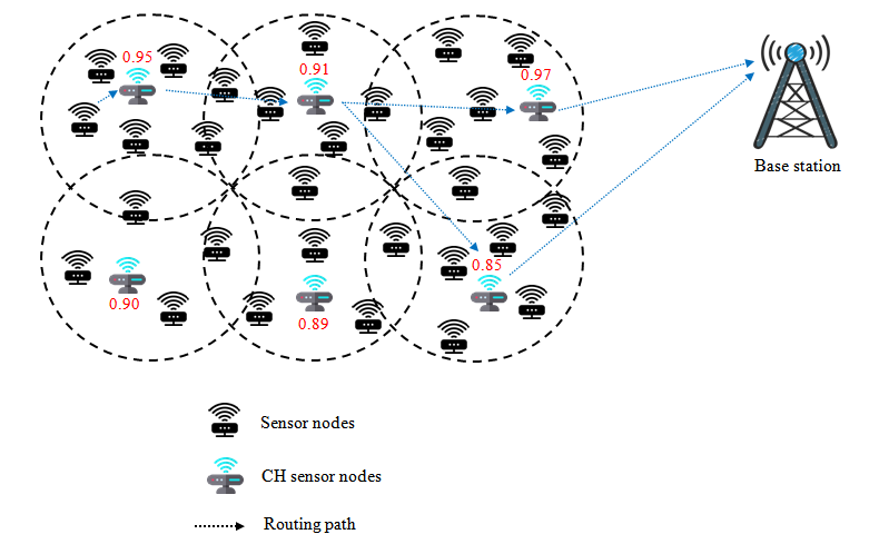
In this proposed model, the different sensors have randomly placed in the network with the emit radiation at approximately square intervals to continuously monitor, as shown in Figure 1. The sensor nodes handle both sensing and receiving data from local network environment. Groups network models and CH selection using a reliable computational model. The path calculation is then computed using a hybrid optimization algorithm.

Figure 1.Cluster based routing network design

Figure 2.Energy consumption with number of nodes

Figure 3.Network lifetime with number of nodes

 

4. Proposed Methodology

In this section, we first discuss the working process of clustering which consist of cluster formation and CH selection. Then, we explain the process of trust computation which is used to compute optimal path.

4.1. Clustering using improved Aquila optimization with fuzzy (IAO-Fuzzy) model

4.1.1. Cluster formation

Aquila Optimizer (AO) is the latest mass intelligence algorithm that reflects Aquila’s hunting techniques for different victims. Faster hunting methods reflect the overall research capabilities of the algorithms, while slower ones utilize the capabilities of the local algorithm. Based on this inspiration, we have developed the improved Aquila optimization (IAO) algorithm used to build teams in this task. The following design parameters are used to create the cluster: location, distance between node-BS, and signal strength received. First, the IAO algorithm starts by defining the initial value of the set of n individuals as follows:

$$\begin{aligned} y_{IJ}&=R_{1} \times\left(u b_{J}-l b_{J}\right)+l b_{J}, \\I&=1,2, \ldots \ldots, \\n J&=1,2, \ldots \ldots, \operatorname{dim} \end{aligned}\tag{1}$$

where $R_{1}$is a random value consisting of ∈ [0, 1]. $lb_{J}$ and $ub_{J}$ Mark the bottom and top edges of the J scale, respectively. Like other transformational technologies, AO has two stages to innovate existing individuals, namely research and exploitation. When the training phase begins $T \leq\left(\frac{2}{3}\right) * t$ there are two modes

$$\begin{aligned} x_{1}(T+1)&=x_{b e s t}(T) \times\left(\frac{1-T}{T}\right) \\&\quad+\left(x_{m}(T)-x_{{best }}(T) * { rand }\right) \end{aligned} \tag{2}$$

where T is the total number of iterations. $x_{b}(T)$ is best recurrence ever obtained in T is the current iteration $\left(\frac{1-T}{T}\right)$, the element used to control the search during the research phase. In addition, $x_{m}(t)$ it is one of the individual averages and is calculated as:

$$x_{m}(T)=\frac{1}{n} \sum_{I=1}^{n} x(T), \quad \forall J=1,2, \ldots, \operatorname{dim}\tag{3}$$

IAO algorithm depends on the use of the Levy flight distribution to renew the existing person according to the following relation.

$$\begin{aligned} x_{2}(T+1)&=x_{{best }}(T) \times { levy }(d) \\&\quad+x_{r}(T)+(Y-X) * { rand } \end{aligned} \tag{4}$$

where $x_{r}$ denotes a random chosen separate. $levy(d)$ refers to the Levy flight delivery defined as:

$$\begin{aligned} {levy}(d)&=S \times \frac{U \times \sigma}{|V|^{1 / \beta}}, \\\sigma&=\left(\frac{\Gamma(1+\beta) \sin e\left(\frac{\pi \beta}{2}\right)}{\Gamma\left(\frac{1+\beta}{2}\right) \times \beta \times 2^{\left(\frac{\beta-1}{2}\right)}}\right) \end{aligned} \tag{5}$$

where $S = 0.01$ and $β = 1.5$ are continuous values, $u$ and $υ$ refer to random numbers produced from$[0, 1]$. In Equation (10), $Y$ and $X$ are used to pretend the spiral outline as,

$$Y=R \times \cos (\theta), X=R \times \sin (\theta)\tag{6}$$

$$\begin{aligned} R&=R_{1}+u \times D_{1}, \\\theta&=-\omega \times d_{1}+\theta_{1}, \\ \theta 1&=\frac{3 \times \pi}{2} \end{aligned} \tag{7}$$

where r1 ∈ [0, 20] is a random value. Smaller values indicate $\omega\ = \ 0.005$ and $u = \ 0.00565.$ It depends on the best solution used $(x_{best})$ and the average individual location $(x_{m})$, which is:

$$\begin{aligned} x_{3}(T+1)&=\left(x_{b e s t}(T) \times x_{m}(T)\right) \\&\quad\times \alpha-{ rand } \\&\quad+((u b-l b) \times { rand }+l b) \times \delta \end{aligned} \tag{8}$$

where rand ∈ [0, 1] denotes random number. α and δ denote the mistreatment alteration parameters. The second exploitation technique depends on $x_{best}$, and excellence function.

$$\begin{aligned} x_{4}(T+1)&={q f} \times x_{{best }}(T)-\left(g_{1} \times x(T) \times { rand }\right. \\&\quad-g_{2} \times { levy }(d)+{ rand } \times g_{1} \end{aligned} \tag{9}$$

where the chief aim of using qf is to equilibrium the search approaches, and it is defined as:

$$q f(T)=T^{\frac{2 \times { rand } ()-1}{(1-t)^{2}}}\tag{10}$$

where $g_{1}$ represents dissimilar motions applied to track the best solution as follows:

$$g_{1}=2 \times { rand }()-1\tag{11}$$

where $g_{2}$ is reduced from 2 to 0, and it is expressed as,

$$g_{2}=2 \times\left(1-\frac{T}{t}\right)\tag{12}$$

where rand characterizes a random charge. The working process of cluster formation is described in Algorithm 1.

Algorithm 1.Cluster formation using improved Aquila optimization

1.	Set the initial value for the parameters of the AO.
2.	Generate initial population X.
3.	Find the best individual $x_{ {best}}(T)$
4.	First exploration method
5.	Update the Xi using $$x_{1}(T+1)=x_{{best }}(T) \times\left(\frac{1-T}{T}\right)+\left(x_{m}(T)-x_{{best }}(T) * {rand }\right),$$
6.	End if
7.	Second exploration method
8.	Update the Xi using Equation $$x_{2}(T+1)=x_{{best }}(T) \times l e v y(d)+x_{r}(T)+(Y-X) * \text { rand },$$
9.	First exploitation $$x_{3}(T+1)=\left(x_{{best }}(T) \times x_{m}(T)\right) \times \alpha-{ rand }+((u b-l b) \times { rand }+l b) \times \delta,$$
10.	second exploitation $$x_{4}(T+1)=q f \times x_{{best }}(T)-\left(g_{1} \times x(T) \times { rand }-g_{2} \times { levy }(d)+ { rand } \times g_{1}\right.$$
11.	Find the fitness values
12.	End if
13.	Return (X best ) values

4.1.2. CH selection

We need the decision making technique for cluster head (CH) selection which need following design metrics are energy consumption, data transfer rate, average quality of data transfer rate and congestion rate. Here, we introduce fuzzy model for CH selection. If we take the N decision criterion (DC) for the decision problem, we need to make a pairing comparison and then, make such a comparison based on the preferences of the decision maker in simple language. Fuzzy model use linguistic terminology to compare ambiguous references to good and bad criteria. The design comparison matrix can be created as a result of comparison as follows.

$$\begin{aligned} \widetilde{a}=\left(\begin{array}{c} D A_{1} \\ D A_{2} \\ \vdots \\ D A_{M} \end{array}\right) &\left[\begin{array}{llll} \widetilde{A}_{11} & \widetilde{A}_{12} & \cdots & \widetilde{A}_{1 N} \\ \widetilde{A}_{21} & \widetilde{A}_{22} & \ddots & \widetilde{A}_{2 N} \\ \vdots & \vdots & & \vdots \\ \widetilde{A}_{M 1} & \widetilde{A}_{M 1} & \cdots & \widetilde{A}_{M N} \end{array}\right] \\&\ \left(\begin{array}{llll} D C_{1} & D C_{2} & \cdots & D C_{N} \end{array}\right) \end{aligned}\tag{13}$$

where $\{DA_{1},DA_{2},...,DA_{M}\}$ is substitute set and $\{DC_{1},DC_{2},...,DC_{N}\}$ is decision matrix with the fixed network area, $\tilde{a}_{IJ}$ depicts fuzzy comparative metrics over J. Furthermore, the better criteria are the worse criteria for ambiguous reference comparisons. The Fuzzy model consists following six stages are,

1. Initialize decision criteria set

This position is governed by the Decision criteria (DC). Suppose there is an “N” final criterion, i.e., $\{DC_{1},DC_{2},...,DC_{N}\}$

2. Compute Best/Worst DC

This position does not require comparison. The decision maker usually sets the best and worst criteria.

3. Use linguistic terminology to better define the ambiguous choice of criteria above all other criteria.

The criteria best defined by the decision maker are compared to all other criteria using the linguist’s terminology. The resulting optimal vector is assumed as follows,

$$\widetilde{a}_{b}=\left(\widetilde{A}_{b 1}, \widetilde{A}_{b 2}, \widetilde{A}_{b 3}, \ldots . ., \widetilde{A}_{b n}\right)\tag{14}$$

where $\widetilde{a}_{b}$ defines optimal vector $\widetilde{A}_{bJ}$, where $\widetilde{A}_{bJ}$ points the ambiguous priority of criterion B for the criterion of best result over all other criteria is J.

4. Use linguistic terminology to determine the vague advantage over the worst of all other criteria.

It is necessary to set ambiguous preferences for all other criteria using the worst language terms mentioned at this stage. This way we get the autumn slow optimal vector.

$$\widetilde{a}_{W}=\left(\widetilde{A}_{W 1}, \widetilde{A}_{W 2}, \widetilde{A}_{W 3}, \ldots, \widetilde{A}_{W n}\right)\tag{15}$$

where $\widetilde{a}_{W}$ defines optimal vector $\widetilde{A}_{WJ}$, which points to J should give vague priority to criteria other than the worst criteria.

5. Define optimal $(\widetilde{A}_{b})$ and $(\widetilde{A}_{W})$

The form of TFNs, $\widetilde{A}_{bJ}$ indicate vague preferences for better standards for others, e.g. $\widetilde{A}_{b J}=\left(p_{b j}, q_{b J}, r_{b J}\right)$. $\widetilde{A}_{wJ}$ denoting uncertainty and options for worst solution from others in the form of TFNs, e.g. $\widetilde{A}_{w J}=\left(p_{J w}, q_{J w}, r_{J w}\right)$. So, we use the equation with the fourth definition. Then, we get a distinctly good vector $(cbTo)$ and a sharp other-bad vector $(coTw)$ as follows.

$$c b T o=c_{b}=\left(C_{b 1}, C_{b 2}, C_{b 3}, \ldots \ldots, C_{b N}\right)\tag{16}$$

$$c o T w=c_{W}=\left(C_{W 1}, C_{W 2}, C_{W 3}, \ldots \ldots, C_{W N}\right)\tag{17}$$

6. Calculate the optimal weights $\left(W_{1}^{*}, W_{2}^{*}, \cdots, W_{N}^{*}\right)$.

The optimal best and worst solution is further filtered using different weight function which can derive from the supreme absolute difference $\mid \frac{W_{b}}{W_{J}}-C_{b J}\mid$ and $\mid \frac{W_{j}}{W_{w}}-C_{W J}\mid$for all J is minimized. The nonlinearly unnatural optimization problematic can be expressed as follows.

$${MinMax}\left\{\left|\frac{W_{b}}{W_{J}}-C_{b J}\right|,\left|\frac{W_{J}}{W_{w}}-C_{J W}\right|\right\}\tag{18}$$

where $\sum_{J} W_{J}=1$ define control variable using $W_{J} \geq 0$, ${ forall } J$. Then, above equation is altered by the subsequent non-linear programming problem.

$${ S.T. }\left\{\begin{array}{l} \left|\frac{W_{b}}{W_{J}}-C_{b J}\right| \leq \xi, { for all } \ J \\ \left|\frac{W_{b}}{W_{J}}-C_{b J}\right| \leq \xi, { forall } \ J \\ \sum_{J} W_{J}=1, \\ W_{J} \geq 0, { forall }\ J \end{array}\right.\tag{19}$$

Finally, the proposed Fuzzy model is used to compute the optimal weight $\left(W_{1}^{*}, W_{2}^{*}, \cdots, W_{N}^{*}\right)$ and the heighted optimal weight is considered as CH of each cluster in the network.

Figure 4.Average hop count with number of nodes

Figure 5.Throughput with number of nodes

4.2. Optimal path selection using hybrid beetle search induced decision making algorithm

For selecting best essential attributes for best optimal path selection, we introduce hybrid beetle search induced decision making (BSDM) algorithm in this paper. Beetle antennae search (BAS) algorithm is naturally understand the process of optimization without knowing the particular type of the function and gradient information. Inspired by the floating optimization algorithm, BSDM further improved the algorithm by forming an individual into a group. Address: Each beetle will be displayed graphically from one G to another or from the BS. Set the Gk Gateway to the BS gateway closest to Gd, indicating that Gd is sending data to Gk. The routing path is drawn in an equation,

$$G_{k}=I\left({SetNextg}\left(G_{k}\right), m\right)\tag{20}$$

where $I(SetNextg(G_{k}),m)$ is an indexing function which returns index of mth gateway from $SetNextg$ and $m=Ceil(U_{i,d}\times|SetNextg(G_{k}|)$. The fitness of routing is evaluated as follows:

$$F { it }_{{Routing }}=Max\left(\frac{C_{1}}{D_{{Total }} * \mathcal{W}_{1}+G_{{Hop }} * \mathcal{W}_{2}}\right)\tag{21}$$

Here, $w (w1, w2) ϵ [0,1]$ and $w1 + w2 = 1, C1$ are proportional constants. $D_{Total}$ is defined as the total length that passes through the gates,

$$D_{{Total }}=\sum_{i=1}^{n} D\left(G_{i}, Nextg\left(G_{i}\right)\right)\tag{22}$$

Additionally, $G_{Hop}$ is defined as the total number of gate hops in the network,

$$G_{H o p}=\sum_{i=1}^{n} NextgCount\left(G_{i}\right) \tag{23}$$

Update Solution: This shows the speed at which the beetle eats $Q_{1}=\big((Q_{i1},Q_{i2},...,Q_{iS})\big)^r$. This shows the individual effects of beetles $X_{1}=\big((X_{i1},X_{i2},...,X_{iS})\big)^r$ and $Q_{1}=\big((X_{g1},X_{g2},...,X_{gS})\big)^r$ thus shows the extreme value of the population. The mathematical model for imitating his behavior is as follows;

$$P_{i s}^{k+1}=P_{i s}^{k}+\rho Q_{i s}^{k}+(1-\rho) \varepsilon_{i s}^{k}\tag{24}$$

when $k$ represents the number of current changes, $Q_{is}$ indicates the velocity of the beetle, $\rho$ denotes the positive constant, and $\epsilon_{is}$ indicates the increase in the beetle’s level motion. Here, the speed formula is mathematically explained as follows;

$$\begin{aligned} Q_{i s}^{k+1}&=\omega Q_{i s}^{k}+c_{1} r_{1}\left(X_{i s}^{k}-P_{i s}^{k}\right) \\&\quad+c_{2} r_{2}\left(X_{g s}^{k}-P_{g s}^{k}\right) \end{aligned} \tag{25}$$

where, $c_{1}$ and $c_{2}$ represent two optimistic constants, $r_{1}$ and $r_{2}$ represents optimal weight with the range of $[0, 1]$ and the inertial optimal weight of $\omega$. In this work, we follow the strategy of reducing the weight of the recession, which is mathematically illustrated as follows;

$$\omega=\omega_{\max }-\frac{\omega_{\max }-\omega_{\min }}{K} * k\tag{26}$$

where, $\omega_{min}$ and $\omega_{max}$ denote the minimum as well as maximum value of $\omega$, $k$ and $K$ denotes the present number of iterations as well as the maximum number of iterations. Here, the decision function is mathematically defined as the incremental function expressed in the following way;

$$\varepsilon_{i s}^{k+1}=\delta^{k} * Q_{i s}^{k} * sign\left(f\left(P_{r s}^{k}\right)-f\left(P_{l s}^{k}\right)\right)\tag{27}$$

At this point, we extend the update resolution to a higher level. Here, $\delta$ degrees indicate size. The search behavior of the right antenna and the left antenna is expressed as follows:

$$P_{r s}^{k+1}=P_{r s}^{k}+Q_{i s}^{k} * d / 2\tag{28}$$

$$P_{l s}^{k+1}=P_{r s}^{k}-Q_{i s}^{k} * d / 2\tag{29}$$

Here, the BSDM algorithm first starts a series of random solutions. The search region is updating its site based on its own search engine, which is currently the best solution. The combination of these two factors can not only accelerate the continuum of population growth, but also subject people to more sustainable local optimization when dealing with multiple issues. The solution will be updated until a better solution or routing path is found. Once the optimal solution is reached, the algorithm will shut down.

Figure 6.Number of dead nodes with number of nodes

Figure 7.Energy consumption with number of simulation rounds

Figure 8.Network lifetime with number of simulation rounds

5. Results and Performance analysis

The effectiveness of the EEC-HO routing protocol has been evaluated using two different simulation scenarios. The result of the proposed EEC-HO routing protocol is compared with existing SPR, SPRwDA and Q-DAEER routing methods. The simulation results of proposed EEC-HO routing protocol is compared with those existing state-of-art protocols different quality metrics.

5.1. Simulation Setup and Scenario

A specific EEC-HO routing protocol runs on the Intel Core i3 processor, installed and tested on a network simulator (NS-2) with 4GB of RAM. We estimate the number of detection nodes as 100, 200, 300, 400 and 500. The 200m × 200m sensitivity zone has approximately multiple sensor nodes. The initial energy levels of the nodes are evenly distributed [2J, 2,5J]. The maximum transmission range of the terminals is estimated at 150 remote units (two). The average remaining WSN power for WSN nodes is 1 J power. Table 2 describes the prototype structure of the proposed system.

• Scenario 1: In this test, we convert the number of sinus nodes from 100 to 500 using the standard network size used to analyze the quality of the data transmission.

• Scenario 2: In this experiment, the number of rounds simulated in the standard detection terminal used to analyze the performance of the EEC-HO routing protocol was changed from 1000 to 5000.

5.2. Comparative analysis

Figure 9.Average hop count with number of simulation rounds

Figure 10.Throughput with number of simulation rounds

Figure 11.Number of dead nodes with number of simulation rounds

5.2.1. Scenario 1: Impact of node density

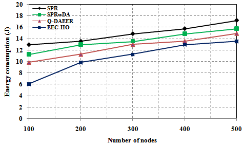
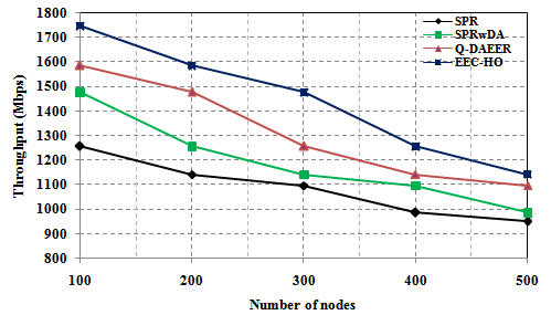
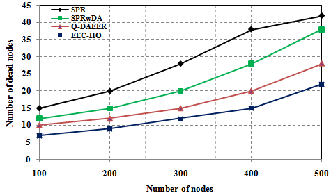
In this scenario, we vary the number of senor nodes as 100, 200, 300, 400 and 500 with the fixed network size as 200m×200m which used to analyze the quality of data transfer. The results of proposed EEC-HO routing protocol is compared with the existing state-of-art protocols are energy consumption, network lifetime, average hop count, throughput and number of dead nodes.

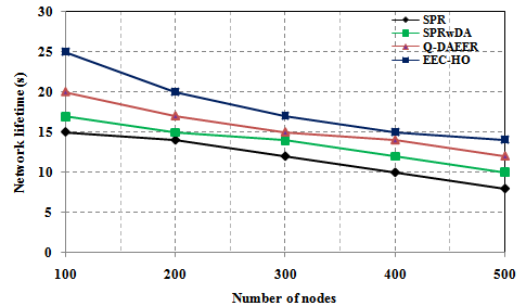
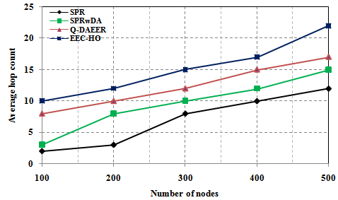
Figure 2 shows a power consumption comparison between the proposed routing protocols and the current protocols. The graph clearly shows that the power consumption of the specified EEC-HO routing protocols is 53.174%, 46.069% and 38.419%, respectively, compared with the SPR, SPRwDA and Q-routing routing protocols. Tire. Figure 3 shows a network lifecycle comparison between specific routing protocols and current protocols. The graph clearly shows that the network life of the proposed EEC-HO routing is 40,000%, 32,000% and 20,000% longer than the related SPR, SPRwDA and Q-DAEER routing protocols. Figure 4 shows the average number of hops and a comparison between the specified routing protocol and the current protocol. The graph clearly shows that the average number of hops for the EEC-HO specific routing is 80,000%, 70,000% and 20,000% higher than the corresponding SPR, SPRwDA and Q-DAEER routing protocols. Figure 5 shows a performance comparison between the proposed routing protocols and the current ones. The graph clearly shows that the routing efficiency recommended by EEC-HO is 28.130%, 15.495% and 9.262% higher than the corresponding SPR, SPRwDA and Q-DAEER routing protocols. Figure 6 shows a comparison of the number of dead nodes between the proposed and existing routing protocols. The graph clearly shows that the number of dead routes of EEC-HO compared with routing protocols SPR, SPRwDA and Q-DAEER is 53.333%, 41.667% and 30,000% respectively.

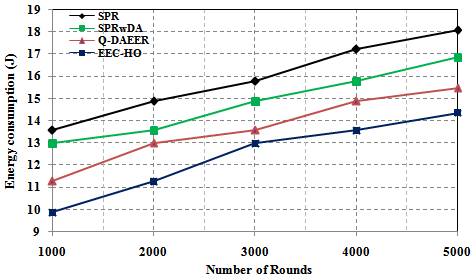
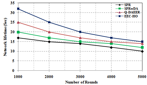
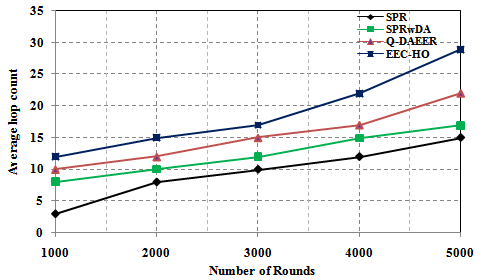
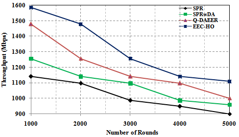
5.2.2. Scenario 2: Impact of Simulation rounds

In this case, the number of simulation circuits used to analyze the performance of the EEC-HO routing protocol will be changed to 1000, 2000, 3000, 4000, 5000 and the standard detection terminal to 500. The results of the proposed EEC-HO routing protocol are compared with existing complex protocols such as power consumption, network life, average hop count, performance, and dead node count. Figure 7 shows a comparison of power consumption between proposed and existing routing protocols. The graph clearly shows that the power consumption of the proposed EEC-HO routing protocols is 27.266%, 23.960% and 12.422% lower, respectively, than the SPR, SPRwDA and Q-router protocols. DAEER. Figure 8 shows a network lifecycle comparison between the proposed routing protocols and the current ones. The graph clearly shows that the network life of the proposed EEC-HO routing is 46.875%, 37.50% and 21.875% longer than the corresponding SPR, SPRwDA and Q-DAEER routing protocols.

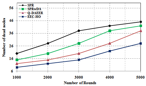
Figure 9 shows the average number of hops and compares the proposed and existing routing algorithms. The graph clearly shows that the average number of hops for the EEC-HO specific routing is 75,000%, 33.333% and 16.667% higher than the related SPR, SPRwDA and Q-DAEER routing protocols. Figure 10 shows a performance comparison between the proposed routing protocols and the current ones. The graph clearly shows that the recommended routing efficiency of EEC-HO is 28.040%, 20.794% and 6.868%, respectively, compared to the routing protocols SPR, SPRwDA and Q-DAEER. Figure 11 shows a comparison of the number of dead nodes between the proposed and existing routing protocols. The graph clearly shows 55,000%, 40,000%, and 25,000% EEC-HO original dead notes compared to SPR, SPRwDA and Q-DAEER routing protocols.

6. Conclusion

We have proposed an energy efficient cluster based routing protocol (EEC-HO) for WSNs using hybrid optimization algorithm. The major contributions of proposed EEC-HO routing protocol is summarized as follows:

• An improved Aquila optimization with fuzzy (IAO-Fuzzy) model is proposed for optimal and efficient cluster formation and cluster head (CH) computation.

• The hybrid beetle search induced decision making algorithm is used for optimal next neighbor selection to transfer data transfer between two nodes.

Finally, we observed that the effectiveness of proposed EEC-HO routing protocol is very effective in terms of energy consumption, network lifetime, average hop count, throughput and number of dead nodes with respect to impact node density and number of simulation scenario respectively.