TRANSFER LEARNING APPROACH FOR CLASSIFICATION OF WIDELY USED SPICES

1.0. Introduction

Spices have been used for centuries in diet and have molecular and biochemical properties that can be used to prevent diseases and treat diseases such as cancer, heart diseases, Alzheimer’s to name a few. The healing properties of spices have been investigated in ¹. Cancer-preventing properties are available in spices such as turmeric, black pepper, garlic, cumin, clove, etc.² Spices are skillfully used by cooks around the world every day to add flavor to the dish and in addition, adding spices will also help in the fight against diseases. The therapeutic property of spices and remedies for many ailments are well documented in ancient Indian books.¹ Many of these Phytonutrients are not available in fruits and vegetables but are available in spices. Spices contain some unique Phytonutrients and other compounds which have anti-oxidant,³ anti-microbial,⁴ and anti-inflammatory powers.⁵ Even though there are numerous spices, this research work concentrates on the classification of the most widely used spices such as turmeric, cumin, pepper, star anise, fenugreek, cardamom, bay leaf, mustard, cinnamon, and cloves.

An investigation of the anticancer property of turmeric which is a common spice in Asian dishes is available in ⁶. The medical application of turmeric has been investigated in ⁷ and it shows turmeric possesses antifungal, antiviral, and anti-venom properties. Cumin is a flowering plant and the dried seeds in the flower are used as a spice by Arabs, Indians, Africans, Americans, Greeks, Egyptians, Romans, and other people in their dishes. The properties of different varieties of cumin are investigated in ⁸ and the investigation reveals cumin has good antioxidant properties. Different varieties of peppercorns are used as a spice and for seasoning. Black pepper, the most common spice is available in shakers in hotels for seasoning. The nutrient composition of different varieties of pepper is analyzed in ⁹. Star anise a spice used for enhancing the flavor of meat and in biryani recipes is also used in perfumes, creams, and pastes in its extracted form. The analysis of the anti-oxygenic property of star-anise is available in ¹⁰. A common ingredient of Indian dishes is cuboid-shaped Fenugreek which is used as a spice to make dal, pickles, sambar (south Indian dish), etc. Therapeutic uses of Fenugreek available in ^11,12 reveals that it can be used as a dietary supplement to cure diabetes. Due to its unique flavor, pleasant aroma, and taste, cardamom has been used in food and beverages from ancient times. The Anti-ulcer properties of cardamom have been researched in ¹³. Dried bay leaf a spice commonly used in soups, gram masala, and biryani for its unique flavor also has therapeutic effects.¹⁴ One of the most commonly used spices in the United States of America; Asian and European countries are mustard seeds. The use of mustard seed powder for alleviation of bladder cancer is investigated in ¹⁵. Aromatic and flavor-rich cinnamon is used in a variety of dishes such as tea, cereals, sweets, and savories, etc. The properties of cinnamon and its role in the treatment of diabetes is analyzed in ¹⁶. Aromatic cloves are used for culinary, non- culinary, and traditional medicinal purposes. The antimicrobial properties of cloves are analyzed in ¹⁷. The literature review of widely used spices indicates they are used in many forms and also have medicinal properties.

Artificial Intelligence (AI) is a technology that makes a machine learn and simulate human behavior using Machine Learning (ML) algorithms and/or Deep Learning algorithms such as Deep Neural Networks (DNN) and Convolutional Neural Networks (CNN) to perceive the environment and take actions.¹⁸ A review of the state-of-the-art Artificial Intelligence (AI) techniques used in revolutionizing the food industry using automation and the advancements made in the agriculture sector towards sustainable food production is available in ¹⁹. Computer vision technology makes a computer mimic a human vision and has been used for a variety of purposes such as image classification, image captioning, object detection, object localization, clustering, video analysis, robotic navigation, and many more.²⁰ Convolutional Neural Networks (CNN) are widely used for image classification. For image classification, the features extracted by the convolutional layers and pooling layers are passed on to a DNN to classify images. CNN with 60 million parameters and with Graphics Processing Unit (GPU) have classified 15 million images of 1000 categories with very high accuracy.²¹ In the food industry, the use of computer vision from harvesting to packing is possible and this technology is being used to maximize profit and quality in the food industry.²² Food computing is an interdisciplinary study that uses compute vision technology for the acquisition and analysis of food data to address food perception and dietary management of health.²³ A review of dietary assessment based on food recognition and volume estimation in ²⁴ reveals many challenges in food image processing technology. Accuracy-related issues while classifying different sized images by inserting a new layer in CNN are provided in ²⁵. Food image classification problem using different architectures of CNN has been attempted on standard food image datasets such as UEC100,²⁶ UEC256,²⁷ Food101,²⁸ and Food251²⁹ in ³⁰. Food image classification with an accuracy of around 80% is obtained using the Food 101 dataset using Alexnet and VGG16 in ³¹. A food classification technique for diabetic patients using CNN with NTUA-Food 2017 dataset with 3248 images is proposed in ³² can classify food into 8 categories based on macronutrient content. CNN based on Residual Network architecture for food image classification using FOOD 475 dataset in ³³ reveal CNN can classify a wide variety of food with a high level of accuracy. CNN based on DenseNet structure for classification of Korean food dataset with 18 categorizes in ³⁴ has been implemented using mobile architecture. Classification of Chicken food dishes in Indonesia using CNN in ³⁵ reveals training process is faster when CNN is used with GPU rather than a CPU. Food image classification on the Indian food dataset using CNN is available in ³⁶, Thai foods dataset is available in ^37,38, and Chinese foods are available in ³⁹. Food and beverage image classification using NutriNet is presented in ⁴⁰. In addition to recognizing food images, a study in ⁴¹ can accurately identify foods in different states such as batons, creamy paste, dice chopped, floured, grated, juiced, julienne, peeled, sliced, wedges and whole. A modified version of Alexnet and GoogLenet has been used to classify images of plants and leaves available in AgriPlant dataset, Folio dataset, and Leafsnap dataset using CNN and bag of visual words in ⁴².

A survey of deep learning techniques used in the food industry in ⁴³ has revealed that deep learning as a tool in food science and engineering has shown tremendous progress and a lot of scope for future applications. An online collection of food images from 1000 restaurants and 12000 food supplies in China is used in ⁴⁴ along with image cleaning and CNN model for cloud-based online multiclass prediction of food images such as meat, vegetables for a food supply chain industry. FOODAI developed by Singapore Management University uses deep learning techniques and can recognize food with confidence levels.^45,46 Review of automatic food recognition system by mobile devices and the steps involved in implementing the system are discussed in detail in ⁴⁷. Many interesting experiments carried out in ⁴⁸ to compare the classification accuracy of humans with CNN reveals that the human vision system is better than CNN for a limited number of food images but CNN outperforms human when trained with a larger dataset.

Magnetic food texture sensor along with principal component analysis (PCA) is used in ⁴⁹ to classify corn snacks, candy, biscuits, and potato snacks based on the texture of the food. Analysis of 1453 food images with 42 categories using K-Nearest Neighbors (KNN) is carried out in ⁵⁰ have revealed an accuracy of around 80%. But traditional methods based on PCA and feature extraction techniques are limited by hardware performance and have a large error in recognition effect. CNN has outperformed other algorithms such as K-Nearest Neighbors, Fuzzy logic, and Ensemble Decision Trees to accurately classify cherry fruit in ⁵¹ and sour lemons in ⁵².

A detailed literature survey indicates there is no dataset available for the classification of spices and this classification task has not been attempted so far. Moreover, most of the papers in the literature have used python for the classification of images but Matlab also has excellent resources for image classification. Hence in this paper, Matlab has been used for the image classification of spices.

Transfer learning is accomplished using pre-trained models such as Visual Geometry Group (VGG),⁵³ GoogLeNet,⁵⁴ ResNet,⁵⁵ Alexnet,²¹ etc. These pre-trained models are trained with millions of images available in the Imagenet database⁵⁶ and were part of the ImageNet Large-Scale Visual Recognition Challenge (ILSVRC).⁵⁷ These pre-trained models can classify thousands of object categories. Compared to building CNN models from scratch, using a transfer learning approach to classify new objects is easier and faster as these models have extracted informative features from a larger dataset. Few strategies can be used for fine- tuning the model⁵⁸ such as

• Retain the architecture and re-training the entire CNN model.

• Train some of the fully connected and feature extraction layers and leave some of the feature extraction layers frozen.

• Retain the architecture and only train the fully connected layer.

Out of the above approaches, the most popular and the one used in this study is to retain the architecture by making changes only to the last fully connected layer and to retrain the entire CNN model. This article proposes a transfer learning approach to classify widely used spices. Three widely used pre-trained models such as Alexnet, VGG16, and GoogLeNet are employed for the classification of spices. Hyperparameter tuning is also employed to optimize the value of the most common hyper-parameters. The performance of each transfer learning approach is compared based on the accuracy of the classification of spices.

2.0. Description of the Spice10 Dataset

One of the important requirements for machine learning is the availability of the dataset to train the machine. For supervised learning, a vast amount of images along with labels are necessary. To identify spices using deep learning models a spice dataset consisting of images of spices and their labels is the most important requirement and at present, the spice dataset is not available. The vast increase of websites, social media, youtube channels related to food content has helped many to share recipes and food images. Some of the ingredients used in these recipes are the spices and these spice images are downloaded from various websites to create the Spice10 dataset with 2000 images consisting of ten different categories of Spices namely bay leaf, cardamom, cinnamon, cloves, cumin, fenugreek, mustard, pepper, star anise, and turmeric. Each category has 200 images. More than 90% of the training images in the Spice10 dataset are low- resolution color images and have a size of less than 20kb. The Spice10 dataset occupies 37MB of space on the hard disk. To test the accuracy of the trained model on unseen images of spices a test folder consisting of 20 images with 2 images for each class is created. This test folder occupies 3.7 MB on the hard disk.

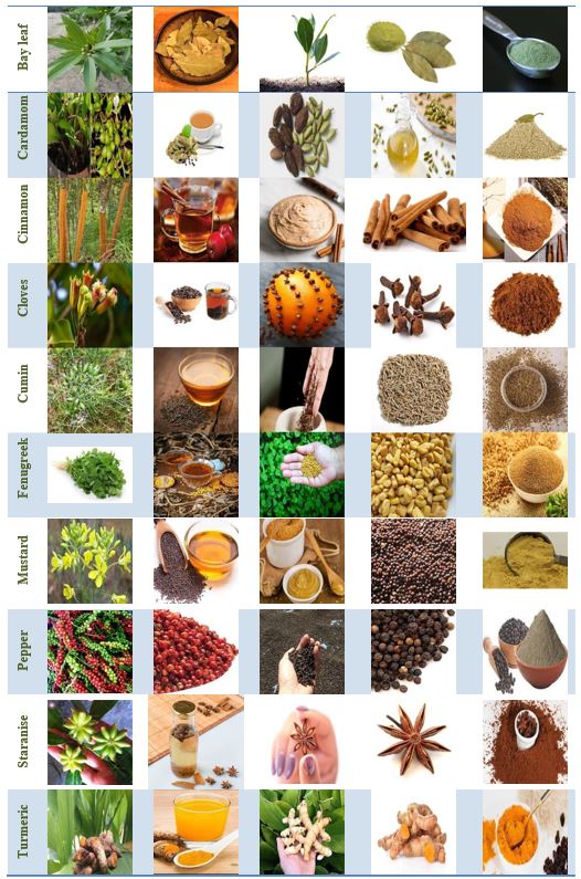
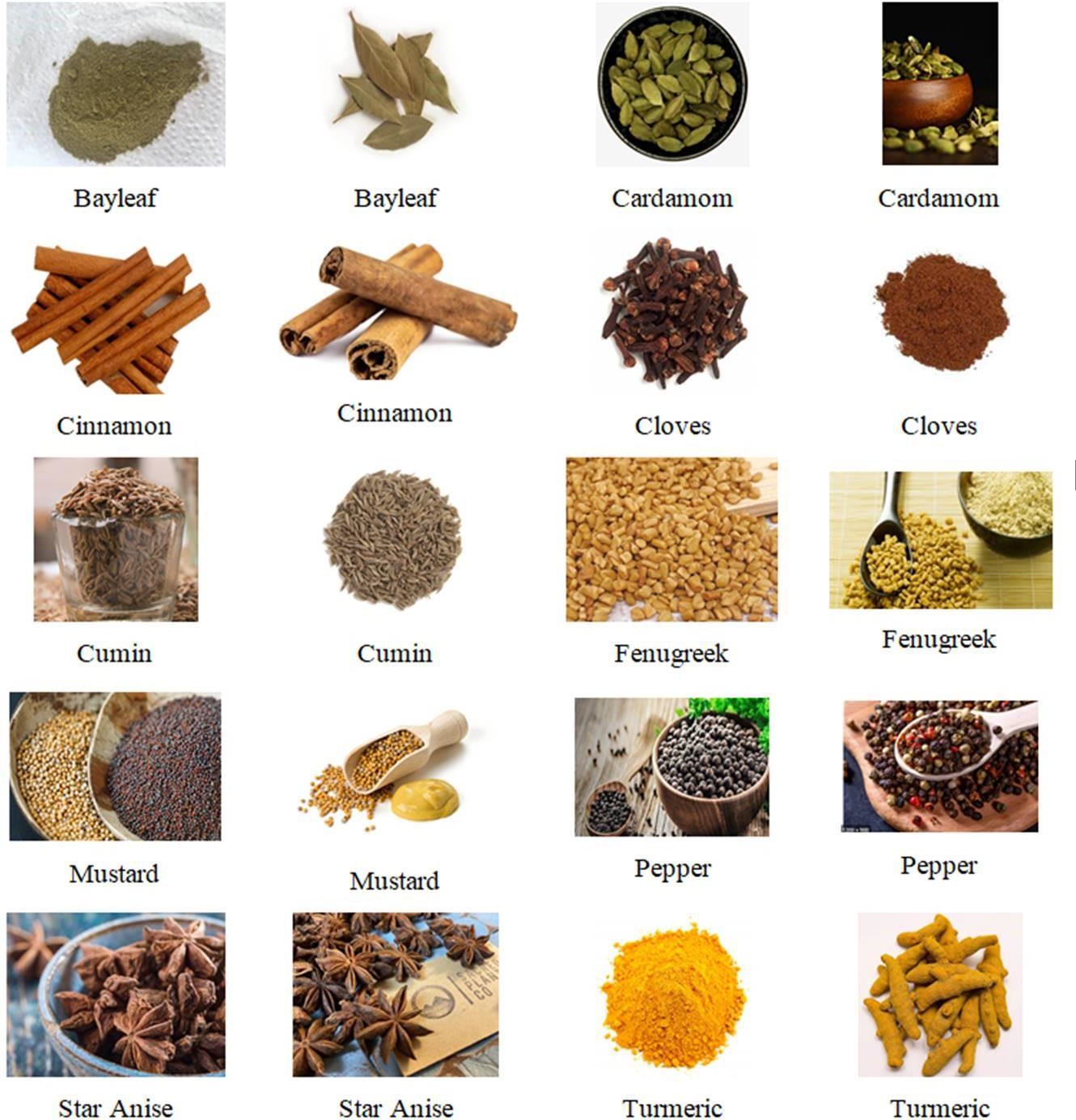
A dataset in a Matlab is referred to as “Datastore”. An imageDatastore in Matlab contains a collection of images and Matlab has the necessary function which also helps us to perform operations such as reading and processing images stored in multiple folders on a disk or in a remote location. Creating labeled data is easy in Matlab as it allows folder name as the label name for the images stored in the folder by using ‘LabelSource’, ‘foldernames’ as name-value pairs when creating the ImageDatastore object. Hence ten subfolders with the names bayleaf ,cardamom, cinnamon, cloves, cumin, fenugreek, mustard, pepper, staranise, and turmeric were created in a folder Spice10. Sample images in the Spice10 dataset are shown in Figure 1.

Figure 1.Sample images in each category of the Spice10 dataset

The first row of Figure 1 shows a sample of bay leaves in the dataset. Fresh bay leaf, dried bay leaf, or grounded forms of bay leaves are commonly used in cooking for their unique aromatic flavors. All these forms of bay leaf are available in the dataset. It is widely used for preparing biryani, gram masala powder, soups, stews, menudo, adobo, massaman curry, and also as a tea infuser. The texture of the bay leaf available in one country is different from other countries. Most often fresh bay leaves are shiny and olive green in color and dried bay leaves are in matte olive green in color.

The second row of Figure 1 shows a sample of cardamom in the dataset. Cardamoms are mostly available in green and black colors are used for flavoring during cooking and also in drinks. Cardamoms are spindle-shaped and when triangular-shaped paper-like pods have opened the seeds inside are in black. Cardamom in its oil form has been used to relieve various stomach issues. Cardamom powders are used in cooking and also in baking. The cardamom with pods, seeds of cardamom, powdered form of cardamom, and cardamom oil are all available in the dataset. The third row of Figure 1 shows a sample of cinnamon in the dataset. Cinnamon is available as a dried bark, as powder, as oil, and as a paste. Cinnamons are used in the preparation of stews, sweets, savories, tea, and also in preparation of medicines. Cinnamon has a medium shade of brown color and is a widely used condiment around the world.

The fourth row of Figure 1 shows a sample of cloves in the dataset. Cloves are aromatic and used in cooking as buds or as powder. Cloves are also used in baking and as pomander by inserting them in oranges. Cloves and clove powder are dark brown with a reddish tinge. Clove available in various forms is part of the dataset. The fifth row of fig 1 shows a sample of cumin in the dataset. Cumin is a dried seed of a plant and is widely used as a whole or in powdered form. Cumin’s are available in brown and black color. Cumin has a distinctive flavor and smell. It is used as part of masala powders, in preparation of some cheese as well as loaves of bread, in soups, and also as a decoction. Cumin as part of decoction, brown cumin, black cumin, powdered form of cumin is all part of the dataset.

The sixth row of fig 1 shows a sample of fenugreek in the dataset. Fenugreek leaves and seeds are used in a variety of cooking. Fenugreek in powdered form is used as a medicine. Leaves are green in color, seeds are angular and brownish-yellow color. The dataset contains the leaves, fenugreek seeds, and powdered form of fenugreek. The seventh row of Figure 1 shows a sample of mustard in the dataset. Mustard is widely used as a condiment to enhance the flavor of the dish. Mustard is used in a variety of forms. Mustard seeds are available in yellowish color to black color are all part of the dataset. Mustard in leafy form, oil form, paste form, and powdered form are all part of the dataset.

The eighth row of Figure 1 shows a sample of pepper in the dataset. Pepper is available in different shapes, forms, and colors. Peppers are used in soups, sauces, stews, marinades, and many other dishes. Peppers in all shapes, forms, and colors are all part of the dataset. The ninth row of fig 1 shows a sample of star anise in the dataset. Star anise is used as a whole or grounded form in cooking and is part of the dataset. The last row of Figure 1 shows a sample of turmeric in the dataset.

Turmeric powders are used in the preparation of a variety of curries and also as food colors. Turmeric rhizome, turmeric powder, turmeric solution are all part of the dataset. From the sample images, it can be inferred that the classification of spices is very complicated as spices in addition to the naturally occurring forms are available in different other forms such as leafy form, powdered or grounded form, as oils, and also as a paste. The machine has to learn the shape of each spice, the various texture of each spice, the different colors of each spice, and must also differentiate a spice that occurs in many forms. The textures of the powdered form of most spices are similar and hence the machine has to differentiate by its color. A small round black mustard and black peppercorn look very similar. The powdered form of cinnamon, star anise, and cloves are all different shades of brown color. Due to all these reasons, it is not easy for a machine to learn all the spices.

3.0. Transfer Learning Approach

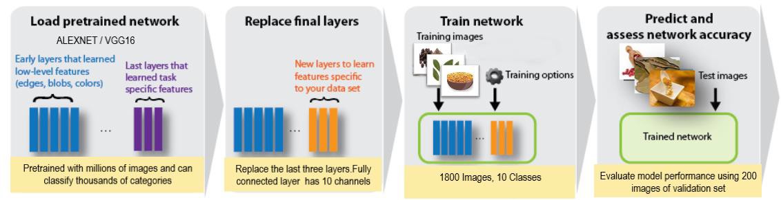
Various deep learning networks have been trained to classify millions of images consisting of thousands of categories. These pre-trained models are generic models that contain vast knowledge of various low and high-level features of the classified images. The transfer learning approach in machine learning uses the knowledge gained while classifying thousands of categories to classify other related images in a new dataset. This is made possible because deep learning can be applied to any domain; features are automatically learned according to the dataset, and due to their property of generalization. Matlab allows fine-tuning the architectures of many pre-trained networks such as Alexnet, VGG16, VGG19, and GoogLeNet. Due to this fine- tuning feature available in Matlab, most of the architecture can be retained and only a few layers may be modified according to the requirement. In this work, Alexnet, GoogLeNet, and VGG 16 have been implemented to classify the images of the spices. The methodology employed in Matlab for image classification of Spice10 dataset is shown in Figure 2.

Figure 2.Transfer learning approach used for classification of spices

The pre-trained Convolution Neural Network (CNN) is many layers deep and comprises manly layers such as convolutional layers, pooling layers, and fully connected layers. Convolutional layers use filter functions to extract features from the images. Convolution is a mathematical transformation of a given function into a form that is more useful than the original function and in image processing convolution is a specialized linear operation while involves scanning the whole image using filters to produce feature maps. CNN works on volumes maintaining spatial structures. Each neuron in CNN receives several inputs and the weighted sum is passed over non-linear activation function such as the rectified linear unit (ReLU), or hyperbolic tangent function. The whole network has a loss function that is optimized using a backpropagation algorithm. Pooling layers are used to remove redundant or low-level features. During pooling, a small feature of the feature map is taken and in that small region, the direction of the strongest gradient (Max Pooling) or the average of the gradient (Average Pooling) is found.

3.1. ALEXNET

Alexnet is an eight-layer deep Convolution Neural Network (CNN) pre-trained on the ImageNet database.⁵⁷ Alexnet can classify millions of images into thousands of categories. Alexnet can be installed in Matlab⁵⁹ and directly applied to classification problems. In this work, the only last three layers of Alexnet are modified according to the Spice10 dataset. The remaining architecture is retained as it is. The number of channels in the last fully connected layer is modified to 10 to match the number of classes of classification in the Spice10 dataset. The modified architecture of Alexnet is shown in Table 1.

The image size for Alexnet is a 227x227x3 input and so spice images have to be resized to 227x227x3 to be used with Alexnet. This is made possible in Matlab by using augmentedImageDatastore function available in Matlab. Alexnet uses five convolutional layers and three fully connected layers. All convolutional layers and the first two fully connected layers use a piecewise linear function called Rectified Linear Unit (ReLU) activation function which outputs a positive value for any positive input otherwise it makes the output zero. The last fully-connected layer uses a normalized exponential function called Softmax and a cross-entropy loss function for multidimensional classification.

Normalization layers, pooling layers, and dropout techniques are also part of Alexnet architecture as seen from Table 1. Cross channel normalization is usually used with the ReLU activation function which is unbounded and detects big neuron response while damping uniformly large responses in the local neighborhood. The dropout technique is used to ignore randomly selected neurons during training to avoid complex co-adaptations during training. Neurons that are randomly selected during dropout do not contribute during the forward propagation of information and backward propagation of error during training the CNN. Pooling is used in Convolutional Neural Networks to remove redundant features. All these techniques are used in Alexnet to learn robust features, improve convergence time, avoid the problems of vanishing gradients, reducing over-fitting, improving generalization, and stabilized training.

3.2. VGG16

One of the best models available today to classify images is the CNN model developed by the Visual Geometry Group (VGG) of Oxford University⁵³ called VGG16 or OxfordNet. VGG16 can be installed in Matlab⁶⁰ and directly applied to classification problems. VGG16 is a huge neural network that has 138 million parameters when compared to 60 million parameters of Alexnet. In this work, only the last three layers of VGG16 are modified according to the Spice10 dataset. The remaining layers are retained as it is. The number of channels in the last fully connected layer is modified to 10 to match the number of classes of classification in the Spice10 dataset. The modified architecture of VGG16 that has sixteen layers is shown in Table 2. The image size for VGG16 is a 224x224x3 input and all images of spices have to be resized to 224x224x3 to be used with VGG16 using augmentedImageDatastore function available in Matlab. All convolutional layers have a 3x3 filter with a stride of 1 and all max-pooling layers

3.3. GoogLeNet

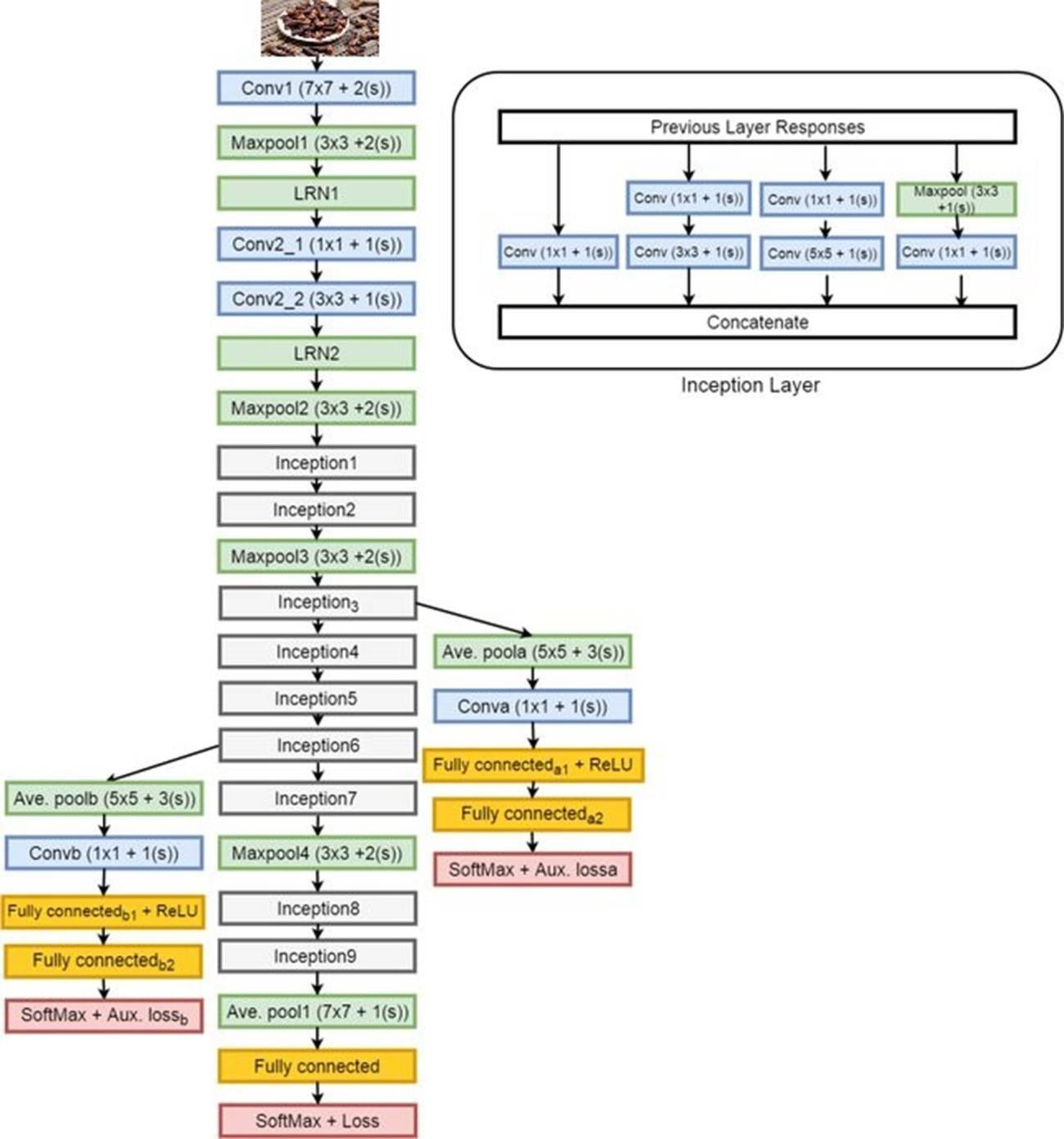
To overcome the problem of overfitting and exploding gradients of architectures with a very high number of layers the researchers in Google used inception modules to develop the GoogLeNet architecture which follows judicious dimension reduction. GoogLeNet architecture consists of 27 layers including 9 inception modules and interested readers can refer to ^54,61 for the detailed description. The input image size for GoogLeNet architecture is 224x224x3 input. 1x1, 3x3, and 5x5 convolutional filters are used in the inception modules to retain important spatial information of the images. A dropout layer with a 40% dropout is used before the linear layer. The linear layer consists of 1000 neurons to classify images into 1000 categories. But, since the Spice10 dataset has only 10 classes the number of neurons is changed to 10 and the entire architecture is retained as it is. The architecture of GoogLeNet is shown in Figure 3.

Figure 3.Architecture of GooLeNet

4.0. Training and Testing of the Models

A transfer learning approach using Alenet, VGG16, and GoogLeNet was implemented in Matlab release 2018b. The training was carried out with HP Pavilion Laptop with Intel (R) Core (TM) i7-8550U CPU @ 1.8 GHz with 16 GB Ram. The first step in the training process is to resize the images to suit the requirements of the pre-trained architecture. This can be easily performed using the imageDataAugmenter object in Matlab. In addition, various other options are also available to rotate, translate, and reflect the images to combat over-fitting. The modified images need not be stored in the computer as the datastore in Matlab which augments the images during training according to the options specified in the imageDataAugmenter object and then discards the images after the training process is complete.

4.1. Hyper Parameter Tunning with Alexnet Architecture

Tuning hyperparameters in machine learning is a very important task as it affects the learning rate of the algorithm, the time complexity of the algorithm, and improves the performance of the algorithm. Normally used approaches for tunning hyperparameters are grid search and random search techniques. But considering the computational complexity involved with very high numbers of hyperparameters to be tunned, in this work coarse-to-fine tunning is adopted to find the optimal set of hyperparameters. In this technique, a random search is carried out to find the promising areas in the search space. This is followed by a deeper search around the promising search space to find the optimal values for hyperparameters. Out of all available well-known architectures, Alexnet has the least number of layers and trainable parameters. Hence the hyperparameter tunning for the Spice10 dataset is carried out in this work using Alexnet architecture.

The most common optimization algorithms used are the adaptive moment estimator (ADAM), stochastic gradient descent (SGD), and root-mean-square propagation (RMSprop). By experimentation it was found SGD with a momentum factor of 0.9 was able to perform better than ADAM and RMSprop. The mini-batch was set as 16 because of limited GPU memory capability and a bigger value caused problems in the convergence of the algorithm. Using the coarse-to-fine technique the optimal values of the hyper-parameters were found as maximum epochs as 15, validation frequency of 50, and validation patience as 5.

The most important hyperparameter is the learning rate. To obtain the best learning rate the learning rate was changed from $1 e^{-3} \ to \ 1 e^{-5}$ to find the performance of the algorithm. 90% of the images in the dataset (1800 images) were used for training and 10% of the images (200 images) in the dataset were used for validation. To find the most important learning rate hyperparameter several experiments were conducted and the results are summarized in Table 3.It was found the network did not learn when the learning rate was set at $1e^{−3}$ which is a case of under-fitting. From the results obtained shown in Table 3, the best learning rate was chosen as $1e^{−4}$ as it was able to produce a better average validation accuracy of 85.5% with a 1.32% standard deviation and lesser training time when compared to a learning rate of $1e^{−5}$.

For the results obtained in Table 3, the number of neurons in the fully connected ‘fc7’ layer shown in Table 1 was 4096. Experiments were also conducted by varying the neurons in the fully connected layer ‘fc7’ shown in Table 1. Experiments were conducted with 2048 and 1024 neurons using the learning rate as $1e^{−4}$. The results of the experiments are shown in Table 4. The results indicate decreasing the number of neurons to 2048 and 1024 does not improve the validation accuracy of the Alexnet model above 85.5% as shown in Table 3 and hence the number of neurons is not changed.

4.2. Results obtained with ALEXNET

Alexnet architecture is loaded into Matlab and the last three layers are modified to match with the Spice10 dataset as shown in Table 1. The Alexnet requires an input size of 227x227x3 but input images in the Spice10 dataset have different sizes and hence augmented image datastore available in Matlab is used to automatically resize the training and validation images to 227x227x3. In addition, the images are rotated by an angle of 20 degrees and also translated by 3 pixels horizontally as well as vertically to avoid over-fitting. The Alexnet was trained using the optimized hyperparameters. The best result obtained during training using optimized hyperparameters is summarized in Table 5.

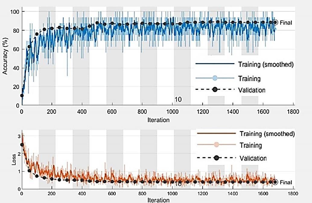
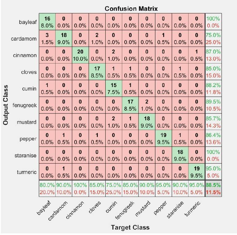
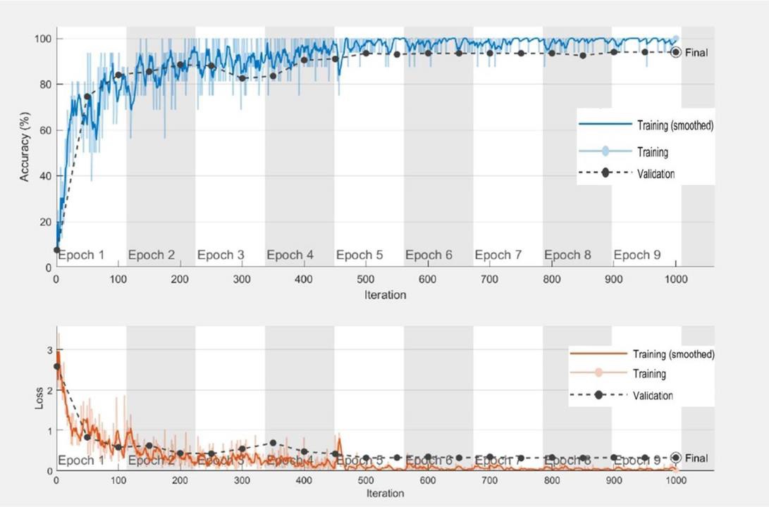
From Figure 4 it can be inferred that when the validation accuracy does not significantly change for 5 epochs the training stops automatically as validation patience was specified as 5 during training. This prevents over-fitting of the model and the validation accuracy of 88.5% indicates that the model will perform at an accuracy of at least 88.5% on the unseen dataset during implementation.

Figure 4.Training Progress for the ALEXNET architecture

Figure 5 shows the confusion chart obtained for the validation set. As seen from the Figure the validation accuracy is 88.5%. The diagonal elements of the confusion chart show the images correctly identified by the Alexnet model. Out of 20 images of Cinnamon in the validation data, the model can identify all of them correctly but for cumin, it can identify only 15 out of the 20 images correctly. Two images of cumin were wrongly identified as cinnamon, two images were wrongly identified as mustard, and one image was wrongly identified as clove.

Figure 5.Confusion Chart obtained for the ALEXNET model with validation data

4.3. Results obtained with VGG16

VGG16 architecture is loaded into Matlab and the last three layers are modified to match with the Spice10 dataset as shown in table 2. The VGG16 requires an input size of 224x224x3 but input images in the Spice10 dataset have different sizes and hence augmented image datastore available in Matlab is used to automatically resize the training and validation images to 224x224x3. In addition, the images are rotated by an angle of 25 degrees and also translated by 3 pixels horizontally as well as vertically to avoid over-fitting. 90% of the images in the dataset were used for training and 10% of the images in the dataset were used for validation. The VGG16 was also trained using the SGD algorithm with the optimized hyperparameters. Validation accuracy obtained during the five runs of the algorithm is summarized in Table 6. TheVGG16 architecture can produce an average validation accuracy of 93.06% which is far higher than Alexnet but has an average time for training is 1 hour 12 minutes which is very high when compared to Alexnet. This time for training is high since the number of trainable parameters is far more when compared to Alexnet.

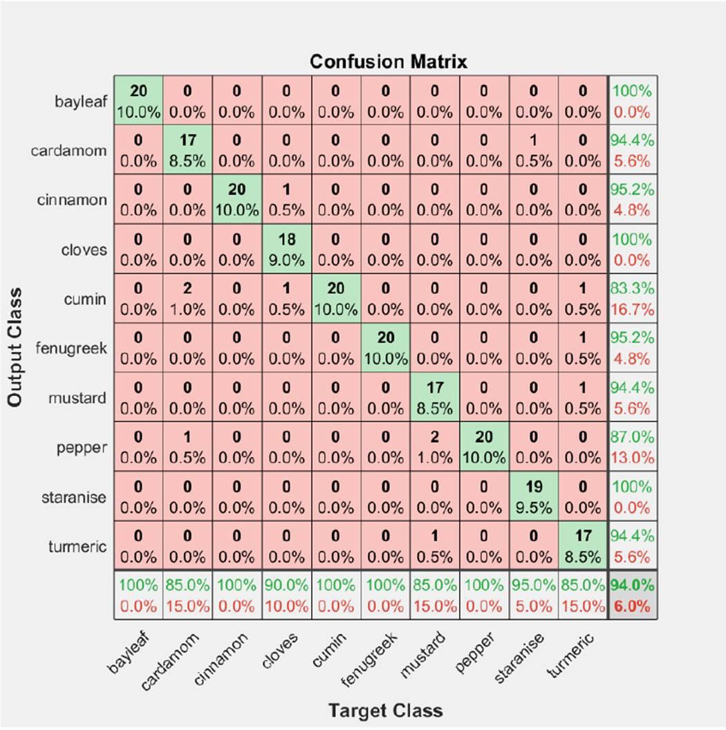
Figure 6 shows the training progress for the best results obtained by VGG16 architecture which is 94% and it can be inferred that when the validation accuracy does not significantly change for 5 epochs the training stops automatically as validation patience was specified as 5 during training. This prevents over-fitting of the model and the validation accuracy of 94 % indicates that the model will perform at an accuracy of at least 94% on the unseen dataset during implementation. Figure 7 shows the confusion matrix obtained for the validation set. As seen from the Figure the validation accuracy is 94%. The diagonal elements of the confusion chart show the images correctly identified by the VGG16 model. The VGG16 model can correctly identify all 20 images of bay leaf, cinnamon, cumin, fenugreek, and pepper available in the validation dataset.

Figure 6.Training progress for the VGG16 architecture.

Figure 7.Confusion Chart obtained for the VGG16 model

4.4. Results obtained with GoogLeNet

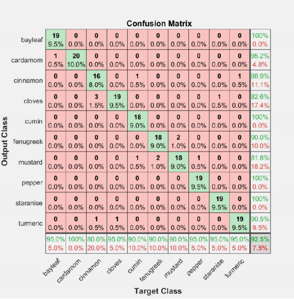
After loading the architecture of GooLeNet in Matlab the images sizes were automatically modified to 224x224x3 using the image datastore function. In addition, the images are rotated by an angle of 25 degrees and also translated by 3 pixels horizontally as well as vertically to avoid over-fitting. 90% of the images in the dataset were used for training and 10% of the images in the dataset were used for validation. The GooLeNet was also trained using the SGD algorithm with the optimized hyperparameters. Validation accuracy obtained during the five runs of the algorithm is summarized in Table 7. Even though GoogLeNet can produce an average validation accuracy of 90.2% it is lesser than the average validation accuracy of the VGG16 model. The confusion chart obtained for the best results of GoogleNet is shown in Figure 8.

Figure 8.Confusion Chart obtained for the GoogLeNet model

4.5. Comparison of results

The summary of the best results obtained with Alexnet, VGG16, and GoogLeNet are summarized in the best table 8. The average validation accuracy obtained by VGG16 is 93.06% which is greater than the average accuracy obtained by Alexnet which is 85.5% and GoogLeNet which is 90.2%. Hence for this Spice10 dataset VGG16 model is preferred over the other two models

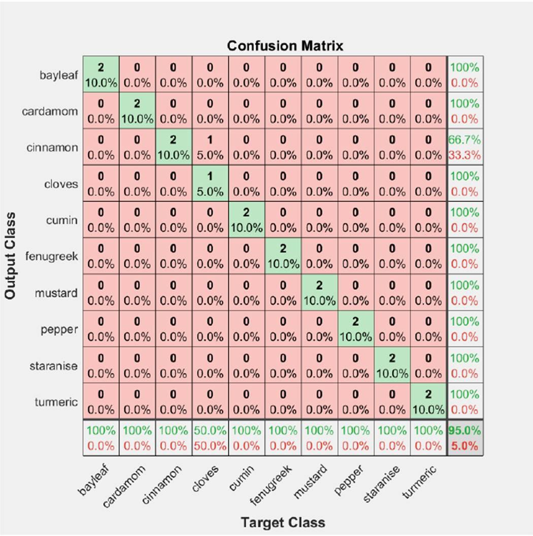
To further check the performance of the VGG16 model on unseen data, 20 images in the test folder shown in Figure 9 were used for classification. Out of twenty images, the model was correctly able to identify 19 images with a testing accuracy of 95%. The confusion chart obtained during testing of the model with an unseen dataset is shown in Figure 10. Only the powdered form of cloves shown in the second row of Figure 8 was wrongly identified as cinnamon by the VGG16 model. This is due to the high similarity in color between cinnamon and cloves.

Figure 9.Images in the test folder of Spice10 dataset

Figure 10.Confusion Chart obtained for the VGG16 model with the test dataset

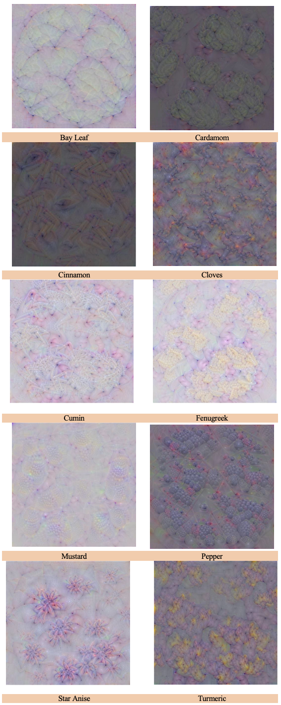
4.6. Feature Map

Features help us to understand the different features learned by the model. The feature map for the fully connected layer obtained for the 10 classes available in the Spice10 dataset is shown in Figure 11 to visualize the features learned for each spice by the VGG16 model. From the feature map, we can infer the model has correctly learned the color, texture, size, and other features of the spices.

Figure 11.Feature maps of the spices using the VGG16 model

6.0. Conclusion

A Spice10 dataset which consists of 2000 images of ten different spices is created in this research work to examine if a machine can classify those images using the transfer learning approach. The classification of spices is a challenging job for a machine as spices are available in many forms, have many similarities in color, shape, and texture. By fine-tuning Alexnet, VGG16, and GoogLeNet architecture, the classification of spices was successfully implemented. The average validation accuracy obtained by the VGG16 model is 93.06% and it can outperform Alexnet and GoogLeNet models. Further, when the VGG16 model was tested on an unseen dataset it was able to produce a testing accuracy of 95%. The high accuracy of the VGG16 model indicates it can be successfully used for the classification of spices.

7.0. Future Work

These datasets can be combined with the existing food dataset to form a large-scale food dataset which will be a vital resource for the development of image classification and recognition algorithm. A larger dataset with many other spices would be trained on a GPU and using the feature maps a mobile application for real-time classification of spices would be developed. An extension of the research work would be to add more spices and research with other pre-trained models.

Acknowledgment

The first author would like to thank the University of Texas at Austin for offering AI and ML courses through Great Learning. The authors would like to acknowledge all support and resources received from the Royal Commission of Jubail and Yanbu for the successful completion of this work. We extend our appreciation to Mrs. Sornalakshmi Arunachalam for her efforts in the preparation of the dataset.